punpy in combination with digital effects tables#

In this section we explain how punpy can be used for propagating uncertainties in digital effects tables through a measurement function. For details on how to create these digital effects tables, we refer to the obsarray documentation. Once the digital effects tables are created, this is the most concise method for propagating uncertainties. The code in this section is just as illustration and we refer to the the CoMet website examples for example with all requied information for running punpy. The punpy package can propagate the various types of correlated uncertainties that can be stored in digital effects tables through a given measurement function. In the next subsection we discuss how these measurement functions need to be defined in order to use the digital effects tables.

Digital Effects Tables#

Digital Effects tables are created with the obsarray package. The documentation for obsarray is the reference for digital effect tables. Here we summarise the main concepts in order to give context to the rest of the Section.

Digital effects tables are a digital version of the effects tables created as part of the FIDUCEO project. Both FIDUCEO effects tables and digital effects tables store information on the uncertainties on a given variable, as well as its error-correlation information (see Figure below). The error-correlation information often needs to be specified along multiple different dimensions. For each of these dimensions (or for combinations of them), the correlation structure needs to be defined. This can be done using an error-correlation matrix, or using the FIDUCEO correlation forms. These FIDUCEO correlation forms essentially provide a parametrisation of the error correlation matrix using a few parameters rather than a full matrix. These thus require much less memory and are typically the preferred option (though this is not always possible as not all error-correlation matrices can be parameterised in this way). Some correlation forms, such as e.g. “random” and “systematic” do not require any additional parameters. Others, such as “triangle_relative”, require a parameter that e.g. sets the number of pixels/scanlines being averaged.

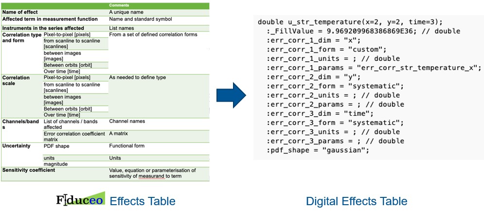
Figure 1 - left: FIDUCEO effects table template. right: obsarray digital effects table for one uncertainty component.

The obsarray package which implements the digital effects tables, extends the commonly used xarray package. xarray objects typically have multiple variables with data defined on multiple dimensions and with attributes specifying additional information. In digital effects tables, each of these variables has one (or more) uncertainty variables associated with it. Each of these uncertainty components is clearly linked to its associated variable, and has the same dimensions. These uncertainty components, unsurprisingly, have uncertainties as the data values. As attributes, they have the information defining the error-correlation structure. If the FIDUCEO correlation forms can be used, the form name and optionally its parameters are stored directly in the attributes of the uncertainty component. If the FIDUCEO correlation forms cannot be used, the form in the attributes is listed as “err_corr_matrix” and as parameter it has the name of another variable in the xarray dataset that has the correlation matrix.

Multiple uncertainty components can be added for the same data variable, and obsarray provide functionality to combine these uncertainties, either as the total uncertainties for a given variable, or as separate random, systematic, and structured components.

Measurement Function#

Generally, a measurement function can be written mathematically as:

\[y = f\left( x_{i},\ldots,\ x_{N} \right)\]

where:

\(f\) is the measurment function;
\(y\) is the measurand;
\(x_{i}\) are the input quantities.

The measurand and input quantities are often vectors consisting of multiple numbers. Here, we choose an example of an ideal gas law equivalent:

\[V = \frac{8.314 \times n T}{P}\]

where:

\(V\) is the volume;
\(n\) is the amount of substance (number of moles);
\(T\) is the temperature;
\(P\) is the pressure.

Here \(V\) is now the measurand, and \(n\), \(T\) and \(P\) are the input quantities. Digital effects tables for \(n\), \(T\) and \(P\) will thus need to be specified prior, and punpy will create a digital effects table for \(V\) as output.

In order to be able to do the uncertainty propagation with these digital effects tables, the measurement functions now need to be defined within a subclass of the MeasurementFunction class provided by punpy. In this subclass, one can then define the measurement function in python as a function called “function”:

from punpy import MeasurementFunction

class GasLaw(MeasurementFunction):
   def function(self, P, T, n):
      return (8.134 * n * T)/P

In some cases, it can also be useful to define the measurand name and input quantity names directly in this class:

from punpy import MeasurementFunction

class GasLaw(MeasurementFunction):
   def function(self, P, T, n):
      return (8.134 * n * T)/P

   def get_measurand_name_and_unit(self):
      return "volume", "m^3"

   def get_argument_names(self):
      return ["pressure", "temperature", "n_moles"]

These names will be used as variable names in the digital effects tables. This means they have to match the expected names in e.g. the input digital effects tables that are used. Providing the names of the input quantities and measurand in this way is not a requirement, as this information can also be provided when initialising the object of this class.

Propagating uncertainties in digital effects tables#

Once this kind of measurement function class is defined, we can initialise an object of this class. In principle there are no required arguments when creating an object of this class (all arguments have a default). However, in practise we will almost always provide at least some arguments. The first argument prop allows to pass a MCPropagation or LPUpropagaion object. It thus specifies whether the Monte Carlo (MC) method (see Section Monte Carlo Method) or Law of Propagation of Uncertainties (LPU) method (see Section Law of Propagation of Uncertainty Method) should be used. These prop objects can be created with any of their options (such as parallel_cores):

prop = MCPropagation(1000, dtype="float32", verbose=False, parallel_cores=4)

gl = IdealGasLaw(prop=prop)

If no argument is provided for prop, a MCPropagation(100,parallel_cores=0) object is used. The next arguments are for providing the input quantity names and the measurand name and measurand unit respectively:

gl = IdealGasLaw(prop=prop, xvariables=["pressure", "temperature", "n_moles"], yvariable="volume", yunit="m^3")

In the xvariables argument, one needs to specify the names of each of the input quantities. These names have to be in the same order as in the specified function, and need to correspond to the names used for the variables in the digital effects tables. These variable names can be provided as optional arguments here, or alternatively using the get_argument_names() function in the class definition. If both options are provided, they are compared and an error is raised if they are different.

Similarly, the yvariable gives the name of the measurand (or list of names if multiple measurands are returned by measurement function) and yunit specifies its associated unit(s). Alternatively, these can also be provided using the get_measurand_name_and_unit() function in the class definition (they will be cross-checked if both are provided). There are many more optional keywords that can be set to finetune the processing of the uncertainty propagation. These will be discussed in the Options when creating MeasurementFunction object section.

Once this object is created, and a digital effects table has been provided (here as a NetCDF file), the uncertainties can be propagated easily:

import xarray as xr
ds_x1 = xr.open_dataset("digital_effects_table_gaslaw.nc")
ds_y = gl.propagate_ds(ds_x1)

This generates a digital effects table for the measurand, which could optionally be saved as a NetCDF file, or passed to the next stage of the processing. The measurand effects table will have separate contributions for the random, systematic and structured uncertainties, which can easily be combined into a single covariance matrix using the obsarray functionalities of the digital effects tables. It is quite common that not all the uncertainty information is available in a single digital effects table. In such cases, multiple digital effects tables can simply be provided to “propagate_ds”. punpy will then search each of these effects tables for the input quantities provided when initialising the MeasurementFunction object. For example, if \(n\), \(T\) and \(P\), each had their own digital effects tables, these could be propagated as:

import xarray as xr
ds_nmol = xr.open_dataset("n_moles.nc")
ds_temp = xr.open_dataset("temperature.nc")
ds_pres = xr.open_dataset("pressure.nc")
ds_y = gl.propagate_ds(ds_pres, ds_nmol, ds_temp)

These digital effects tables can be provided in any order. They can also contain numerous other quantities that are not relevant for the current measurement function. When multiple of these digital effects tables have a variable with the same name (which is used in the measurement function), an error is raised.

functions for propagating uncertainties#

In the above example, we show an example of using the propagate_ds() function to obtain a measurand effects table that has separate contributions for the random, systematic and structured uncertainties. Depending on what uncertainty components one is interested in, there are a number of functions that can be used: * propagate_ds: measurand digital effects table with separate contributions for the random, systematic and structured uncertainties. * propagate_ds_tot: measurand digital effects table with one combined contribution for the total uncertainty (and error correlation matrix). * propagate_ds_specific: measurand digital effects table with separate contributions for a list of named uncertainty contributions provided by the user. * propagate_ds_all: measurand digital effects table with separate contributions for all the individual uncertainty contributions in the input quantities in the provided input digital effects tables.

It is worth noting that the uncertainty components labelled in the measurand digital effect tables as “random” or “systematic” (either in propagate_ds, propagate_ds_specific or propagate_ds_all), will contain the propagated uncertainties for all uncertainty components on the input quantities that are random or systematic respectively along all the measurand dimensions. Any uncertainty components on the input quantities where this is not the case (e.g. because the error correlation along one dimension is random and along another is systematic; or because one of the error correlations is provided as a numerical error correlation matrix) will be propagated to the structured uncertainty components on the measurand.

This is somewhat further complicated by the fact that the input quantity dimensions are not always the same as the measurand dimensions. If any of the measurand dimensions is not in the input quantity dimensions, some assumption needs to made about how this input quantity will be correlated along that measurand dimension. Often, such a situation will simply mean that the same value of the input quantity will be used for every index along the measurand dimension (broadcasting). This often leads to a systematic correlation along this measurand dimension (a typical example would be the same spectral gains being applied to multiple spectral scans in a measurement, where the gains have a wavelength dimension and the spectral scans have wavelength and scan index dimensions; any error in the gains, will affect all scans equally). There are however also scenarios where the introduced error-correlation along the measurand dimension should be random (e.g. if a constant temperature is assumed and applied along the time dimension, but we know in reality the temperature is fluctuating randomly w.r.t. to assumed temperature). It can also be structured. Detailed understanding of the problem is thus required when the measurand dimensions are not present along the measurand dimensions. By default, punpy assumes that the error correlation along the missing dimensions is systematic. If another error correlation is required, this can be done by setting the expand keyword to True and the broadcast_correlation to the appropriate error correlation (either “rand”, “syst” or an error correlation matrix as a numpy array). Depending on how this broadcast error correlation combines with the error correlations in the other dimensions, can also affect which measurand uncertainty component (random, systematic or structured) it contributes to when using propagate_ds.

Sometimes one wants to propagate uncertainties one input quantity at a time. This can be the case no matter if we are propagating total uncertainties or individual components. When creating the MeasurementFunction object, it is possible to specify on which input quantities the uncertainties should be propagated using the uncxvariables keyword:

gl = IdealGasLaw(prop=prop,
                  xvariables=["pressure", "temperature", "n_moles"],
                  uncxvariables=["pressure"]
                  yvariable="volume",
                  yunit="m^3")
ds_y = gl.propagate_ds(ds_pres, ds_nmol, ds_temp)

In the above example, only the uncertainties on pressure will be propagated. This behaviour could also be obtained by removing the unc_comps in the temperature and n_moles variables in their respective datasets, but the solution shown above is easier. If no uncxvariables are provided, the uncertainties on all input quantities are propagated.

Options when creating MeasurementFunction object#

A number of additional options are available when creating the MeasurementFunction object, and when running one of the propagate_ds functions. We refer to the API for a full list of the keywords, but here highlight some of the ones that were not previously explained.

When creating the MeasurementFunction object, we previously discussed the prop, xvariables, uncxvariables, yvariable and yunit keywords. Next, there are a number of keywords that are the same as the keywords for using punpy as standalone. These are corr_between,`param_fixed`, repeat_dims, corr_dims, seperate_corr_dims, allow_some_nans. Here these keywords work in the same way as for standalone punpy and we refer to the Punpy as a standalone package Section for further explanation. The one difference is that here, the repeat_dims and corr_dims can be provided as dimension names rather than dimension indices (dimension indices are also still allowed). If a string corr_dim is provided that is present in some but not all of the measurand dimensions (only relevant when there are multiple differently-shaped measurands), the seperate_corr_dims will automatically be set to True, and the appropriate separate corr_dims will be worked out automatically.

The options we have not previously explained are the ydims, refxvar and sizes_dict. These all have to do with the handling of dimensions when they differ between input quantities (or between input quantities and measurand). In the typical punpy usecase, the dimensions of the measurand are the same as the dimensions of the input quantities. If this is not the case, the ydims keyword should be set to a list of the measurand dimensions (in order matching the shape). If one of these dimensions is not in the input quantities, one should also provide sizes_dict, which is a dictionary with all dimension names as keys, and the dimension size as the value. Alternatively, if the dimensions of the measurand match the dimensions of one (but not all) of the input quantities, the measurnad shape can be automatically set if refxvar is provided, where refxvar is the name of the input quantity with matching shape.

Finally the use_err_corr_dict is explained in the Managing memory and processing speed in punpy Section.

Options when running propagate_ds functions#

There are also a few options when running the propagate_ds (or similar) functions. The store_unc_percent keyword simply indicates whether the measurand uncertainties should be stored in percent or in the measurand units (the latter is the default). The expand keyword indicate whether the input quantities should be expanded/broadcasted to the shape of the measurand, prior to passing to the measurement function (defaults to False).

ds_out_pre allows to provide a pre-generated xarray dataset (typically made using obsarray) in which the results will be stored. This can be used to add additional variables to the dataset prior to running the uncertainty propagation, or to concatenate multiple uncertainty propagation results into one file. By default, the measurand variables and associated uncertainty and error correlation will be overwritten, but all other variables in the dataset remain. If one does not want to get punpy to work out the error correlations iteself, but just use the ones in the template (e.g. because in complex cases, punpy can run into problems), this can be specified by setting the use_ds_out_pre_unmodified keyword to True. In this case, only the values of the variables will be changed, but none of the attributes.

Finally the include_corr keyword can be set to False if error correlations should be omited from the calculation. The latter results in faster processing but can lead to wrong results so should be used with caution.

punpy in combination with digital effects tables

Contents