
Algorithm Theoretical Basis#
Principles of Uncertainty Analysis#
The Guide to the expression of Uncertainty in Measurement (GUM 2008) provides a framework for how to determine and express the uncertainty of the measured value of a given measurand (the quantity which is being measured). The International Vocabulary of Metrology (VIM 2008) defines measurement uncertainty as:
“a non-negative parameter characterizing the dispersion of the quantity values being attributed to a measurand, based on the information used.”
The standard uncertainty is the measurement uncertainty expressed as a standard deviation. Please note this is a separate concept to measurement error, which is also defined in the VIM as:
“the measured quantity value minus a reference quantity value.”
Generally, the “reference quantity” is considered to be the “true value” of the measurand and is therefore unknown. Figure 1 illustrates these concepts.
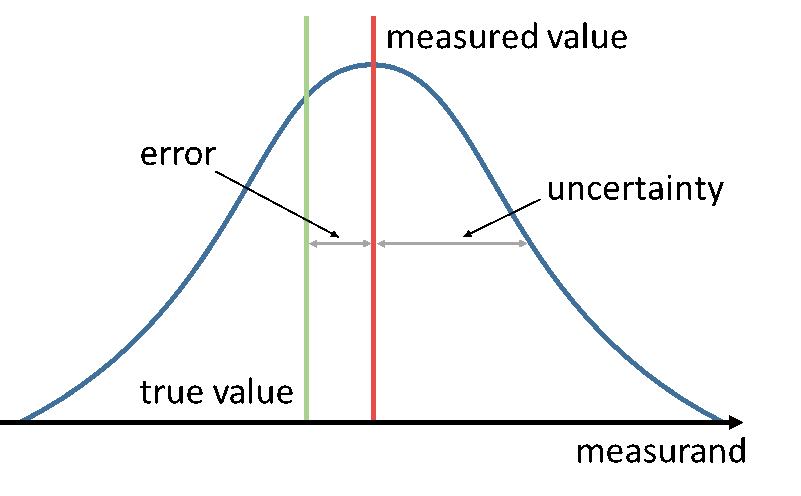
Figure 1 - Diagram illustrating the different concepts of measured value and true value, uncertainty and error.
In a series of measurements (for example each pixel in a remote sensing Level 1 (L1) data product) it is vital to consider how the errors between the measurements in the series are correlated. This is crucial when evaluating the uncertainty of a result derived from these data (for example a Level 2 (L2) retrieval of geophysical parameter from a L1 product). In their vocabulary the Horizon 2020 FIDUCEO [1] (Fidelity and uncertainty in climate data records from Earth observations) project (see FIDUCEO Vocabulary, 2018) define three broad categories of error correlation effects important to satellite data products, as follows:
Random effects: “those causing errors that cannot be corrected for in a single measured value, even in principle, because the effect is stochastic. Random effects for a particular measurement process vary unpredictably from (one set of) measurement(s) to (another set of) measurement(s). These produce random errors which are entirely uncorrelated between measurements (or sets of measurements) and generally are reduced by averaging.”
Structured random effects: “means those that across many observations there is a deterministic pattern of errors whose amplitude is stochastically drawn from an underlying probability distribution; “structured random” therefore implies “unpredictable” and “correlated across measurements”…”
Systematic (or common) effects: “those for a particular measurement process that do not vary (or vary coherently) from (one set of) measurement(s) to (another set of) measurement(s) and therefore produce systematic errors that cannot be reduced by averaging.”
Law of Propagation of Uncertainty Method#
Within the GUM framework uncertainty analysis begins with understanding the measurement function. The measurement function establishes the mathematical relationship between all known input quantities (e.g. instrument counts) and the measurand itself (e.g. radiance). Generally, this may be written as
where:
\(Y\) is the measurand;
\(X_{i}\) are the input quantities.
Uncertainty analysis is then performed by considering in turn each of these different input quantities to the measurement function, this process is represented in Figure 2. Each input quantity may be influenced by one or more error effects which are described by an uncertainty distribution. These separate distributions may then be combined to determine the uncertainty of the measurand, \(u^{2}(Y)\), using the Law of Propagation of Uncertainties (GUM, 2008),
where:
\(\mathbf{C}\) is the vector of sensitivity coefficients, \(\partial Y/\partial X_{i}\);
\(\mathbf{S(X)}\) is the error covariance matrix for the input quantities.
This can be extended to a measurement function with a measurand vector (rather than scalar) \(\mathbf{Y}=(Y_{i},\ldots,\ Y_{N})\). The uncertainties are then given by:
where:
\(\mathbf{J}\) is the Jacobian matrix of sensitivity coefficients, \(J_{ni} = \partial Y_{n}/\partial X_{i}\);
\(\mathbf{S(Y)}\) is the error covariance matrix (n*n) for the measurand;
\(\mathbf{S(X)}\) is the error covariance matrix (i*i) for the input quantities.
The error covariances matrices define the uncertainties (from the diagonal elements) as well as the correlation between the different quantities (off-diagonal elements).
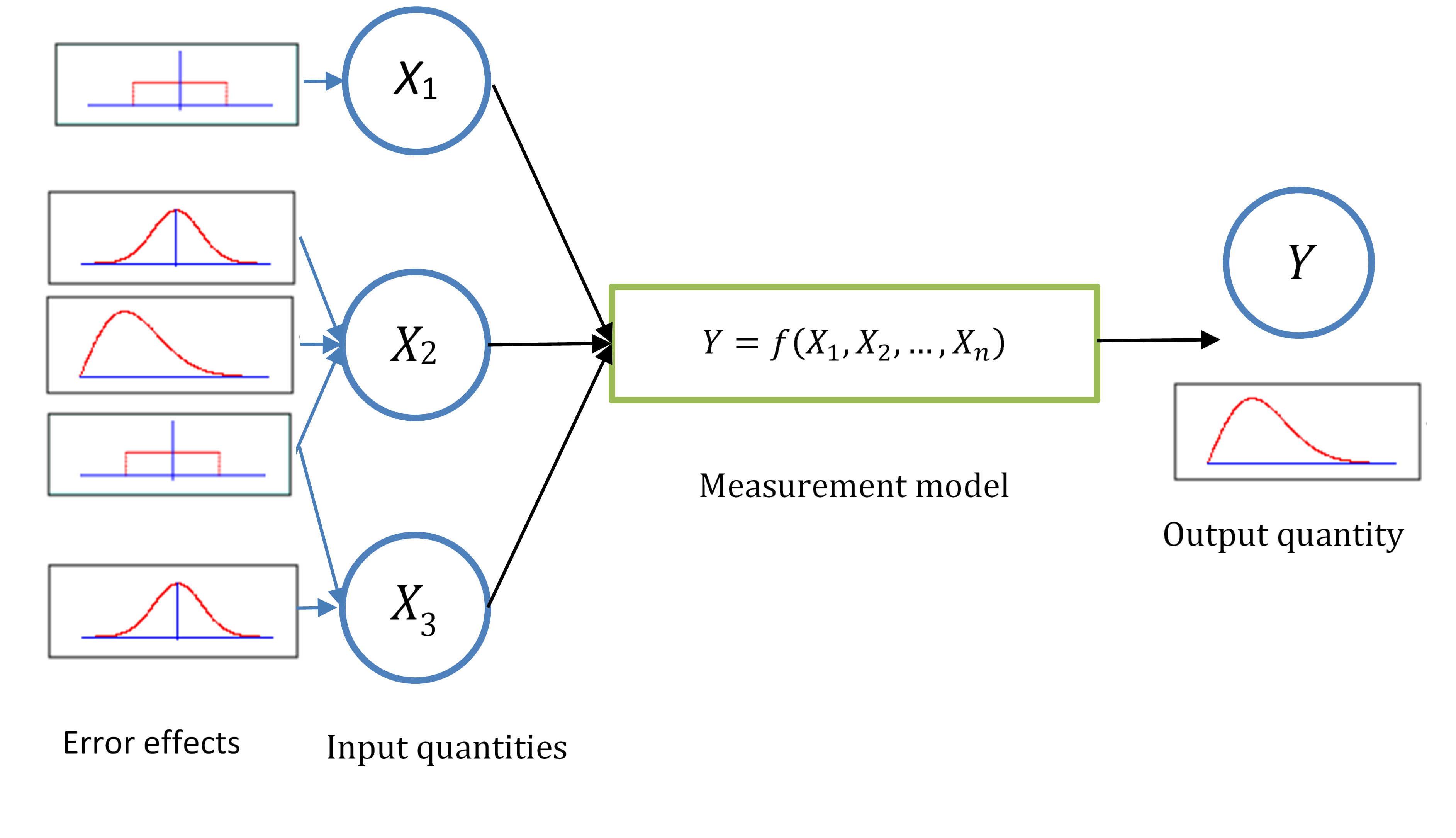
Figure 2 - Conceptual process of uncertainty propagation.
Monte Carlo Method#
For a detailed description of the Monte Carlo (MC) method, we refer to Supplement 1 to the “Guide to the expression of uncertainty in measurement” - Propagation of distributions using a Monte Carlo method.
Here we summarise the main steps and detail how these were implemented. The main stages consist of:
Formulation: Defining the measurand (output quantity Y), the input quantities \(X = (X_{i},\ldots,\ X_{N})\), and the measurement function (as a model relating Y and X). One also needs to asign Probability Density Functions (PDF) of each of the input quantities, as well as define the correlation between them (through joint PDF).
Propagation: propagate the PDFs for the \(X_i\) through the model to obtain the PDF for Y.
Summarizing: Use the PDF for Y to obtain the expectation of Y, the standard uncertainty u(Y) associated with Y (from the standard deviation), and the covariance between the different values in Y.
The MC method implemented in punpy consists of generating joint PDF from the provided uncertainties and correlation matrices or covariances. Punpy then propagates the PDFs for the \(X_i\) to Y and then summarises the results through returning the uncertainties and correlation matrices.
As punpy is meant to be widely applicable, the user can define the measurand, input quantities and measurement function themselves. Within punpy, the input quantities and measurand will often be provided as python arrays (or scalars) and the measurement function in particular needs to be a python function that can take the input quantities as function arguments and returns the measurand.
To generate the joint PDF, comet_maths is used. The ATBD for the comet_maths PDF generator is given here.
The measurand pdf is then defined by processing each draw \(\xi_i\) to Y:
\(Y = f(\xi)\).
The measurands for each of these draws are then concatenated into one array containing the full measurand sample. The uncertainties are than calculated by taking the standard deviation along these draws.
When no corr_dims are specified, but return_corr is set to True, the correlation matrix is calculated
by calculating the Pearson product-moment correlation coefficients of the full measurand sample along the draw dimension.
When corr_dims are specified, the correlation matrix is calculated along a subset of the full measurand sample.
This subset is made by taking only the first index along every dimension that is not the correlation dimension.
We note that corr_dims should only be used when the error correlation matrices do not vary along the other dimension(s).
A warning is raised if any element of the correlation matrix varies by more than 0.05 between the one using a subset taking
only the first index along each other dimension and the one using a subset taking only the last index along each other dimension.